4 The Modified Euler Method
The Euler method can be effective when it comes to solving differential equations numerically but on occasions, the global error of \(\mathcal{O}\left(h\right)\) is rather poor. The Euler method can modified and improved to give Modified or Improved Euler Method (also known as the Heun Method, named after Karl Heun).
4.1 Steps of the Modified Euler Method
The Modified Euler Method utilises the Fundamental Theorem of Calculus which states that for a differentiable function \(y\) defined on the interval \([t_0,t_1]\) (where \(t_1=t_0+h\) for some stepsize \(h\)), \[y(t_1)-y(t_0)=\int\limits_{t_0}^{t_1} \! y'(t) \; \mathrm{d} t.\] In the interval \([t_0,t_1]\), the derivative \(y'(t)\) may be approximated by the derivative at the leftmost point \(y'(t_0)\), this approximation forms the basis of the standard Euler method; \[\begin{align*} y(t_1)-y(t_0) & =\int\limits_{t_0}^{t_1} \! y'(t) \; \mathrm{d} t \\ & =\int\limits_{t_0}^{t_1} \! y'(t_0) \; \mathrm{d} t \\ & =h y'(t_0) \end{align*}\] \[\implies \quad y(t_1)=y(t_0)+hy'(t_0).\]
However, if \(y'(t)\) varies substantially then this approximation can lead to some poor predictions. This can be modified so rather than approximating \(y'(t)\) by \(y'(t_0)\) only, it can be approximated by taking an average between \(y'(t_0)\) and \(y'(y_1)\), namely \[y'(t) \approx \frac{1}{2}\left( y'(t_0)+y'(t_1) \right).\] Thus \[\begin{align*} y(t_1)-y(t_0) & =\int\limits_{t_0}^{t_1} \! y'(t) \; \mathrm{d} t \\ & =\int\limits_{t_0}^{t_1} \! \frac{1}{2}\left( y'(t_0)+y'(t_1) \right) \; \mathrm{d} t \\ & = \frac{h}{2}\left( y'(t_0)+y'(t_1) \right) \end{align*}\] \[\implies \quad y(t_1)=y(t_0)+\frac{h}{2}\left( y'(t_0)+y'(t_1) \right).\]
Initially, one might suspect that the derivative \(y'(t_1)\) can be found from the differential equation itself, namely, \(y'(t_1)=f(t_1,y(t_1))\) but to do that, a Prediction-Correction procedure needs to be employed where the Euler method can be used to predict a value of \(y(t_1)\) and this is then corrected afterwards. This is done as follows: \[\begin{align*} \bullet \quad \text{Predictor:} \quad & \tilde{Y}_{n+1}=Y_n+h f(t_n,Y_n) \\ \bullet \quad \text{Corrector:} \quad & Y_{n+1}=Y_n+\frac{h}{2} \left[ f(t_n,Y_n)+f(t_{n+1},\tilde{Y}_{n+1}) \right]. \end{align*}\]
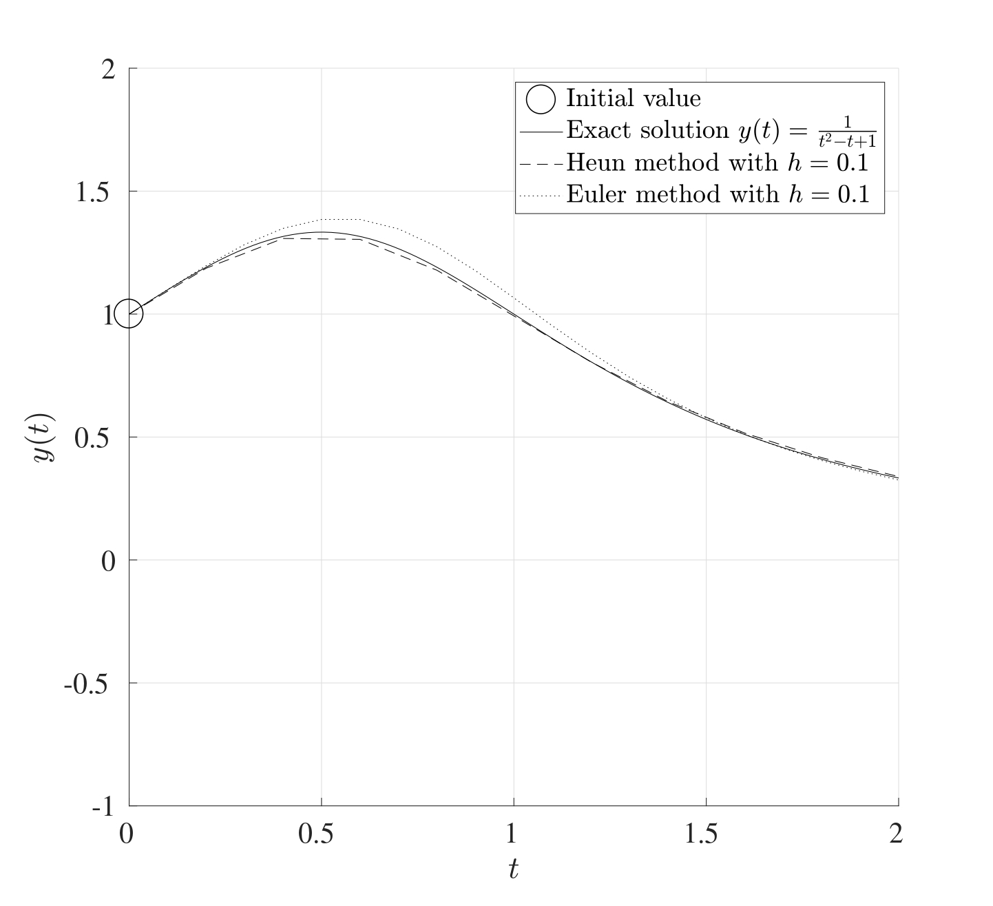
Consider the differential equation \[\frac{\mathrm{d} y}{\mathrm{d} t}=(1-2t)y^2 \quad \text{with} \quad y(0)=1, \quad t\in [0,2].\] This differential equation is non-linear but has a known particular solution which is \[y(t)=\frac{1}{t^2-t+1}\] and this will be compared to the approximate solutions obtained from the standard and Modified Euler methods.
The figure below shows how the standard and modified Euler methods compare to the exact solution for the same stepsize \(h=0.1\). This suggests that the Modified Euler method has improved accuracy compared to the Euler method for the same stepsize, however as a consequence, the function \(f\) on the right hand side of the differential equation has to be calculated twice for every step; once in the prediction stage and once for the correction. However even with this in mind, doubling the number of calculations to improve accuracy can also warrant for a coarser choice of the stepsize to allow for a more efficient use of computational time.
4.2 Accuracy of the Modified Euler Method
In order to asses the accuracy of the Modified Euler method, consider the Taylor series expansion of \(y\) at the points \(t_0\) and \(t_1\) about \(t_{0.5}=t_0+\frac12 h\):
\[y(t_1)=y\left( t_{0.5}+\frac{h}{2} \right)=y(t_{0.5})+\frac{h}{2}y'(t_{0.5})+\left( \frac{h}{2} \right)^2 \frac{1}{2!} y''(t_{0.5})+\mathcal{O}\left(h^3\right),\] \[y(t_0)=y\left( t_{0.5}-\frac{h}{2} \right)=y(t_{0.5})-\frac{h}{2}y'(t_{0.5})+\left( \frac{h}{2} \right)^2 \frac{1}{2!} y''(t_{0.5})+\mathcal{O}\left(h^3\right).\]
Subtracting \(y(t_0)\) from \(y(t_1)\) gives \[y(t_1)-y(t_0)=hy'(t_{0.5})+\mathcal{O}\left(h^3\right). \tag{4.1}\]
The Taylor series expansion can also be done for the derivative of \(y\) at the points \(t_0\) and \(t_1\) about \(t_{0.5}=t_0+\frac12 h\) in a similar way as above, i.e. \[y'(t_1)=y'\left( t_{0.5}+\frac{h}{2} \right)=y'(t_{0.5})+\frac{h}{2}y''(t_{0.5})+\mathcal{O}\left(h^2\right),\] \[y'(t_0)=y'\left( t_{0.5}-\frac{h}{2} \right)=y'(t_{0.5})-\frac{h}{2}y''(t_{0.5})+\mathcal{O}\left(h^2\right).\] Adding \(y'(t_0)\) to \(y'(t_1)\) gives \[y'(t_1)+y'(t_0)=2y'(t_{0.5})+\mathcal{O}\left(h^2\right),\] thus multiplying by \(\frac{h}{2}\) and using equation Equation 4.1 yields \[\frac{h}{2}\left[ y'(t_1)+y'(t_0) \right]=y(t_1)-y(t_0)+\mathcal{O}\left(h^3\right). \tag{4.2}\]
The first step of the Modified Euler method is to predict the value of \(y'(t_1)\) using the Euler iteration; \[\tilde{Y}_1=\underbrace{y(t_0)+h y'(t_0)}_{\approx y(t_1)}+\mathcal{O}\left(h^2\right).\] Hence \[y'(t_1)=f(t_1,y(t_1))\approx f(t_1,\tilde{Y}_1)+\mathcal{O}\left(h^2\right).\] All this information can now be used to obtain the improved update \(Y_1\) which is the corrected form of \(\tilde{Y}_1\). Thus from equation Equation 4.2, \[\underbrace{y(t_1)}_{\approx Y_1} =\underbrace{y(t_0)}_{=Y_0}+ \frac{h}{2}[ \underbrace{y'(t_1)}_{=f(t_1,\tilde{Y}_1)}+\underbrace{y'(t_0)}_{=f(t_0,Y_0)}]+\mathcal{O}\left(h^3\right)\] \[\implies \quad Y_1=Y_0+\frac{h}{2}\left[ f(t_1,\tilde{Y}_1)+f(t_0,Y_0) \right]. \tag{4.3}\]
Equations Equation 4.3 and Equation 4.2 can be used to find the local truncation error for the Modified Euler method at the first time step which is \[e=\left| y(t_1)-Y_1 \right|=\left| y(t_1)-\left[ y(t_0)+\frac{h}{2}\left( y'(t_1)+y'(t_0) \right) \right]\right|+\mathcal{O}\left(h^3\right)=\mathcal{O}\left(h^3\right).\] Therefore the local truncation error \(e=\mathcal{O}\left(h^3\right)\) meaning that the Modified Euler method is third order accurate which is an improvement over the Euler method.
The global integration error can be obtained just as before to show that the global integration error of the Modified Euler method is \(E=\mathcal{O}\left(h^2\right)\) meaning that this is a second order method. In particular, if the stepsize \(h\) is halved, the global integration error will be reduced by a factor of four while the local truncation error will reduce by a factor of eight.
4.3 MATLAB Code
The following MATLAB code performs the Modified Euler iteration for the following set of IVPs on the interval \([0,1]\): \[\begin{align*} & \frac{\mathrm{d} u}{\mathrm{d} t}=2u+v+w+\cos(t), & \quad u(0)=0 \\ & \frac{\mathrm{d} v}{\mathrm{d} t}=\sin(u)+\mathrm{e}^{-v+w}, & \quad v(0)=1 \\ & \frac{\mathrm{d} w}{\mathrm{d} t}=uv-w, & \quad w(0)=0. \end{align*}\]
Note that this code is built for a general case that does not have to be linear even though the entire derivation process was built on the fact that the system is linear.
function IVP_Mod_Euler

%% Solve a set of first order IVPs using Modified Euler

% This code solves a set of IVP when written explicitly
% on the interval [t0,tf] subject to the initial conditions
% y(0)=y0.  The output will be the graph of the solution(s)
% and the vector value at the final point tf.  Note that the
% IVPs do not need to be linear or homogeneous.

%% Lines to change:

% Line 28   : t0 - Start time
% Line 31   : tf - End time
% Line 34   : N  - Number of subdivisions
% Line 37   : y0 - Vector of initial values
% Line 116+ : Which functions to plot, remembering to assign
%             a colour, texture and legend label
% Line 130+ : Set of differential equations written
%             explicitly.  These can also be non-linear and
%             include forcing terms.  These equations can
%             also be written in matrix form if the
%             equations are linear.

%% Set up input values

% Start time
t0=0;

% End time
tf=1;

% Number of subdivisions
N=5000;

% Column vector initial values y0=y(t0)
y0=[0;1;0];

%% Set up IVP solver parameters

% T = Vector of times t0,t1,...,tN.
% This is generated using linspace which splits the
% interval [t0,tf] into N+1 points (or N subintervals)
T=linspace(t0,tf,N+1);

% Stepsize
h=(tf-t0)/N;

% Number of differential equations
K=length(y0);

%% Perform the Modified Euler iteration

% Y = Solution matrix
% The matrix Y will contain K rows and N+1 columns.  Every
% row corresponds to a different IVP and every column
% corresponds to a different time.  So the matrix Y will
% take the following form:
% y_1(t_0)  y_1(t_1)  y_1(t_2)  ...  y_1(t_N)
% y_2(t_0)  y_2(t_1)  y_2(t_2)  ...  y_2(t_N)
% ...
% y_K(t_0)  y_K(t_1)  y_K(t_2)  ...  y_K(t_N)
Y=zeros(K,N+1);

% The first column of the vector Y is the initial vector y0
Y(:,1)=y0;

% Set the current time t to be the starting time t0 and the
% current value of the vector y to be the strtaing values y0
t=t0;
y=y0;

for n=2:1:N+1

    % Prediction Step:
    % Use the Euler iteration to obtain an appromxation for
    % the derivatives at the current time step

    dydt=DYDT(t,y,K);     % Find gradient at the current step
    y_pred=y+h*dydt;   % Predict y at current time step

    % Corrector Step:
    % Use the Modified Euler to correct y_pred

    dydt_pred=DYDT(t,y_pred,K);    % Predict the gradient
    % from the predicted y
    y=y+0.5*h*(dydt+dydt_pred); % Find y at the current step

    t=T(n);            % Update the new time

    Y(:,n)=y;          % Replace row n in Y with y

end

%% Setting plot parameters

% Clear figure
clf

% Hold so more than one line can be drawn
hold on

% Turn on grid
grid on

% Setting font size and style
set(gca,'FontSize',20,'FontName','Times')
set(legend,'Interpreter','Latex')

% Label the axes
xlabel('$t$','Interpreter','Latex')
ylabel('$\mathbf{y}(t)$','Interpreter','Latex')

% Plot the desried solutions.  If all the solutions are
% needed, then consider using a for loop in that case
plot(T,Y(1,:),'-b','LineWidth',2,'DisplayName','$y_1(t)$')
plot(T,Y(2,:),'-r','LineWidth',2,'DisplayName','$y_1(t)$')
plot(T,Y(3,:),'-k','LineWidth',2,'DisplayName','$y_1(t)$')

% Display the values of the vector y at tf
disp(strcat('The vector y at t=',num2str(tf),' is:'))
disp(Y(:,end))

end

function [dydt]=DYDT(t,y,K)

% When the equation are written in explicit form

dydt=zeros(K,1);

dydt(1)=2*y(1)+y(2)+y(3)+cos(t);

dydt(2)=sin(y(1))+exp(-y(2)+y(3));

dydt(3)=y(1)*y(2)-y(3);

% If the set of equations is linear, then these can be
% written in matrix form as dydt=A*y+b(t).  For example, if
% the set of equations is:
% dudt = 7u - 2v +  w + exp(t)
% dvdt = 2u + 3v - 9w + cos(t)
% dwdt =      2v + 5w + 2
% Then:
% A=[7,-2,1;2,3,-9;0,2,5];
% b=@(t) [exp(t);cos(t);2];
% dydt=A*y+b(t)

end