5 Fourth Order Runge-Kutta Method
The Modified Euler method extended the Euler method to a two-stage procedure with a global integration error of \(\mathcal{O}\left(h^2\right)\). This can be extended further to a Multi-Stage Method, also called a Runge-Kutta Method with \(p\) stages and a global error integration error of \(\mathcal{O}\left(h^p\right)\) for any arbitrarily large \(p\) (in this case, the Modified Euler method is known as a second order Runge-Kutta method since it has two stages). For instance, the fourth order Runge-Kutta method requires four calculations for every step and has a global integration error of \(\mathcal{O}\left(h^4\right)\), this is formulated as follows: \[\begin{align*} K_1 & = f(t_n, Y_N), \\ K_2 & = f\left( t_n+\frac{h}{2}, Y_n+\frac{h}{2}K_1 \right),\\ K_3 & = f\left( t_n+\frac{h}{2}, Y_n+\frac{h}{2}K_2 \right),\\ K_4 & = f\left( t_{n+1}, Y_n+hK_3 \right)\\ Y_{n+1} & = Y_n +\frac{h}{6}\left[ K_1+2K_2+2K_3+K_4 \right]. \end{align*}\]
Runge-Kutta methods like this are quite versatile and are generally the most used methods for their accuracy since the stepsize \(h\) does not need to be too small to achieve good results. Even though every step requires four calculations, the value of \(h\) can be made larger in order to reduce the cost but retain considerable accuracy.
Consider the differential equation \[\frac{\mathrm{d} y}{\mathrm{d} t}=y(1-2t) \quad \text{where} \quad y(0)=1, \quad t \in [0,3.2].\] The exact solution to this differential equation is known to be \[y(t)=\mathrm{e}^{t(1-t)}.\]
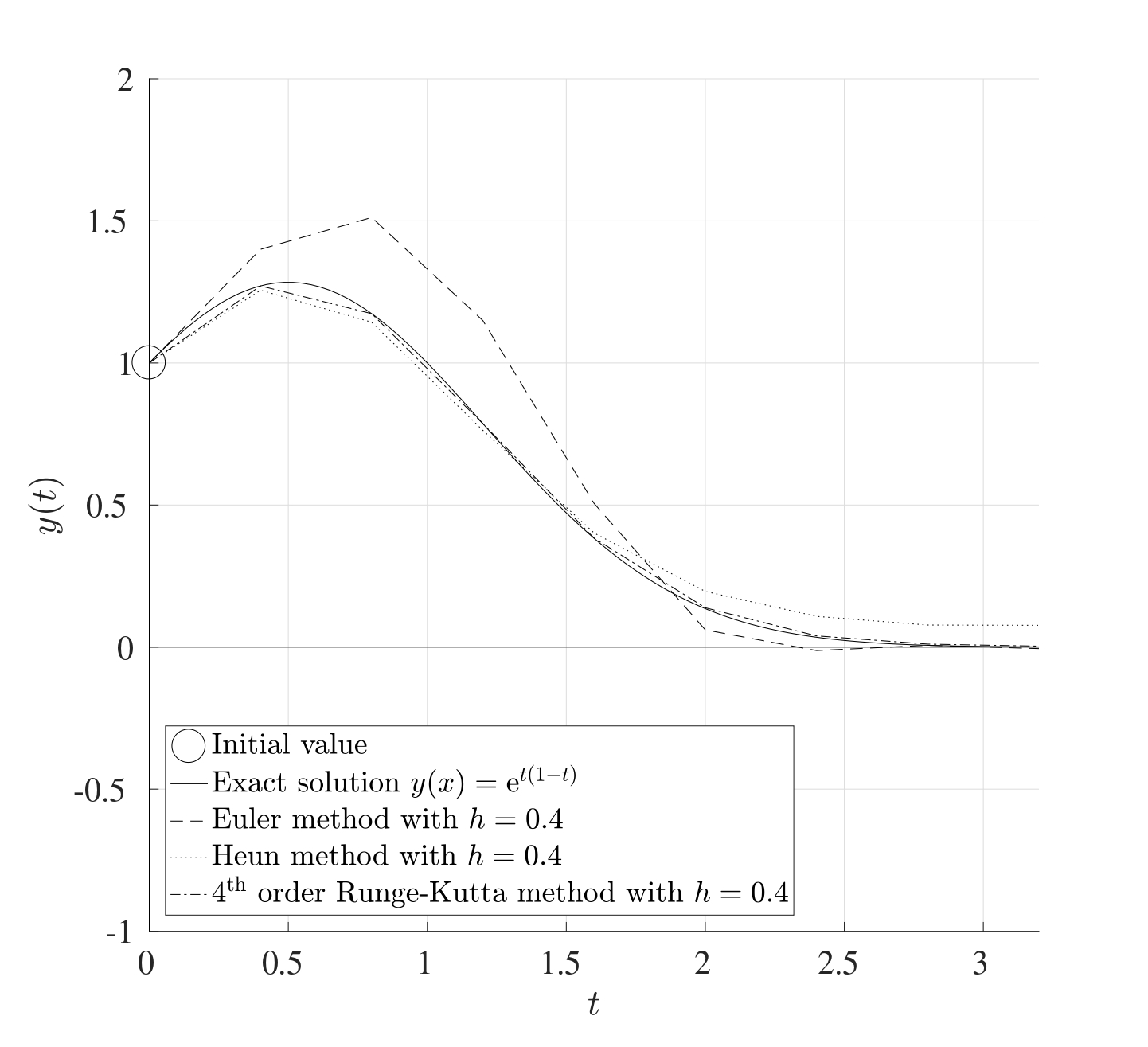
The figure above shows the exact solution to the differential equation (solid line) with the three different methods used to approximate the solution all at the same resolution of \(h=0.4\). The stepsize \(h\) is quite coarse but this is merely for the purposes of demonstration. The Euler method is the least accurate for this coarse grid, the Heun method improves the accuracy while the fourth order Runge-Kutta method is the most accurate out of the three even for the same stepsize.
5.1 MATLAB Code
The following MATLAB code performs the fourth order Runge-Kutta iteration for the following set of IVPs on the interval \([0,1]\): \[\begin{align*} & \frac{\mathrm{d} u}{\mathrm{d} t}=2u+v+w+\cos(t), & \quad u(0)=0 \\ & \frac{\mathrm{d} v}{\mathrm{d} t}=\sin(u)+\mathrm{e}^{-v+w}, & \quad v(0)=1 \\ & \frac{\mathrm{d} w}{\mathrm{d} t}=uv-w, & \quad w(0)=0. \end{align*}\]
Note that this code is built for a general case that does not have to be linear even though the entire derivation process was built on the fact that the system is linear.
function IVP_RK4

%% Solve a set of first order IVPs using RK4

% This code solves a set of IVP when written explicitly
% on the interval [t0,tf] subject to the initial conditions
% y(0)=y0.  The output will be the graph of the solution(s)
% and the vector value at the final point tf.  Note that the
% IVPs do not need to be linear or homogeneous.

%% Lines to change:

% Line 28   : t0 - Start time
% Line 31   : tf - End time
% Line 34   : N  - Number of subdivisions
% Line 37   : y0 - Vector of initial values
% Line 110+ : Which functions to plot, remembering to assign
%             a colour, texture and legend label
% Line 124+ : Set of differential equations written
%             explicitly.  These can also be non-linear and
%             include forcing terms.  These equations can
%             also be written in matrix form if the
%             equations are linear.

%% Set up input values

% Start time
t0=0;

% End time
tf=1;

% Number of subdivisions
N=50;

% Column vector initial values y0=y(t0)
y0=[0;1;0];

%% Set up IVP solver parameters

% T = Vector of times t0,t1,...,tN.
% This is generated using linspace which splits the
% interval [t0,tf] into N+1 points (or N subintervals)
T=linspace(t0,tf,N+1);

% Stepsize
h=(tf-t0)/N;

% Number of differential equations
K=length(y0);

%% Perform the RK4 iteration

% Y = Solution matrix
% The matrix Y will contain K rows and N+1 columns.  Every
% row corresponds to a different IVP and every column
% corresponds to a different time.  So the matrix Y will
% take the following form:
% y_1(t_0)  y_1(t_1)  y_1(t_2)  ...  y_1(t_N)
% y_2(t_0)  y_2(t_1)  y_2(t_2)  ...  y_2(t_N)
% ...
% y_K(t_0)  y_K(t_1)  y_K(t_2)  ...  y_K(t_N)
Y=zeros(K,N+1);

% The first column of the vector Y is the initial vector y0
Y(:,1)=y0;

% Set the current time t to be the starting time t0 and the
% current value of the vector y to be the strtaing values y0
t=t0;
y=y0;

for n=2:1:N+1

    % Determine the coefficients of RK4

    K1=DYDT(t,y,K);
    K2=DYDT(t+h/2,y+h*K1/2,K);
    K3=DYDT(t+h/2,y+h*K2/2,K);
    K4=DYDT(t+h,y+h*K3,K);
    y=y+(h/6)*(K1+2*K2+2*K3+K4);

    t=T(n);            % Update the new time

    Y(:,n)=y;          % Replace row n in Y with y

end

%% Setting plot parameters

% Clear figure
clf

% Hold so more than one line can be drawn
hold on

% Turn on grid
grid on

% Setting font size and style
set(gca,'FontSize',20,'FontName','Times')
set(legend,'Interpreter','Latex')

% Label the axes
xlabel('$t$','Interpreter','Latex')
ylabel('$\mathbf{y}(t)$','Interpreter','Latex')

% Plot the desried solutions.  If all the solutions are
% needed, then consider using a for loop in that case
plot(T,Y(1,:),'-b','LineWidth',2,'DisplayName','$y_1(t)$')
plot(T,Y(2,:),'-r','LineWidth',2,'DisplayName','$y_2(t)$')
plot(T,Y(3,:),'-k','LineWidth',2,'DisplayName','$y_3(t)$')

% Display the values of the vector y at tf
disp(strcat('The vector y at t=',num2str(tf),' is:'))
disp(Y(:,end))

end

function [dydt]=DYDT(t,y,K)

% When the equation are written in explicit form

dydt=zeros(K,1);

dydt(1)=2*y(1)+y(2)+y(3)+cos(t);

dydt(2)=sin(y(1))+exp(-y(2)+y(3));

dydt(3)=y(1)*y(2)-y(3);

% If the set of equations is linear, then these can be
% written in matrix form as dydt=A*y+b(t).  For example, if
% the set of equations is:
% dudt = 7u - 2v +  w + exp(t)
% dvdt = 2u + 3v - 9w + cos(t)
% dwdt =      2v + 5w + 2
% Then:
% A=[7,-2,1;2,3,-9;0,2,5];
% b=@(t) [exp(t);cos(t);2];
% dydt=A*y+b(t)

end