9 Mixed Value Problems
Initial and boundary value problems are not the only two ways in which conditions can be expressed. Sometimes these conditions can be presented in a mixed form where the condition on one or both boundaries may depend on the derivative of the solution function. For instance, consider the steady-state convection-diffusion equation on a bar on length \(5\) with density \(\rho\), convective velocity \(v\), specific heat capacity \(C_p\), thermal conductivity \(k_f\) and heat source \(f\): \[-k_f \frac{\mathrm{d}^{2} T}{\mathrm{d} x^{2}}+\rho v C_p \frac{\mathrm{d} T}{\mathrm{d} x}=f(x) \quad \text{on} \quad x \in [0,5] \quad \text{with} \quad T(0)=100 \quad \text{and} \quad \frac{\mathrm{d} T}{\mathrm{d} x}(5)=0\] where \(T(x)\) is the temperature at \(x\). This set of conditions are known as Mixed Conditions: the first \(T(0)=100\) means that the temperature at the location \(x=0\) is \(100\), the second \(\frac{\mathrm{d} T}{\mathrm{d} x}(5)=0\) means that at the location \(x=5\), there is no heat flux. This can be quite useful if say, a metal rod is being heated to \(100^{\circ}\)C on one side an insulated on the other.
The method to solving MVPs is the same as boundary value problems subject to a few modifications.
9.1 Finite Difference Method for MVPs
Consider the differential equation \[a(x) \frac{\mathrm{d}^{2} u}{\mathrm{d} x^{2}}+b(x) \frac{\mathrm{d} u}{\mathrm{d} x}+c(x) u=f(x) \quad \text{with} \quad 0< x < L\] as before. The interval \([0,L]\) will be split into \(N\) equally sized sections each of width \(h=\frac{L}{N}\) and the grid points are labelled \(x_n=nh\) for \(n=0,1,2,\dots,N\). This differential equation can be discretised using the centred difference approximation just as before to give \[\alpha_n U_{n-1}+\beta_n U_n+\gamma_n U_{n+1}=f(x_n) \quad \text{for} \quad n=1, 2, \dots, N-1\] \[\text{where} \quad \alpha_n=\frac{a(x_n)}{h^2}-\frac{b(x_n)}{2h}, \quad \beta_n=-\frac{2a(x_n)}{h^2}+c(x_n), \quad \gamma_n=\frac{a(x_n)}{h^2}+\frac{b(x_n)}{2h}.\] This gives a set of \(N-1\) equations in \(N+1\) unknowns, namely \(U_0, U_1, U_2, \dots, U_N\) (recall that \(U_n \approx u(x_n)\) for \(n=0, 1, 2, \dots, N\)).
When the differential equation is subjected to two boundary conditions, say \[u(0)=u_l \quad \text{and} \quad u(L)=u_r,\] then expressions for \(U_0\) and \(U_L\) are provided which gives \(N-1\) equations in \(N-1\) unknowns, hence resulting in a well-defined system which can be solved as before.
However, suppose that a set of mixed conditions is given as \[\frac{\mathrm{d} u}{\mathrm{d} x}(0)=\tilde{u}_l \quad \text{and} \quad u(L)=u_r.\] In this case, only \(U_N \approx u(L)=u_r\) is explicitly known, meaning that there will be \(N-1\) equations in \(N\) unknowns since \(U_0 \approx u(x_0)\) is not known giving an under-determined system (a system with more unknowns than equations). So either one more equation is needed or one more unknown needs to be removed. All the unknowns are certainly needed, otherwise the solution will be incomplete, so the alternative is to find another equation to add to the set of equations.
The set of \(N-1\) equations is: \[\begin{align*} n=1: & \quad \alpha_1 U_0+\beta_1 U_1+\gamma_1 U_{2}=f(x_1) \\ n=2: & \quad \alpha_2 U_{1}+\beta_2 U_2+\gamma_2 U_{3}=f(x_2) \\ & \qquad \qquad \qquad \vdots \\ n=N-1: & \quad \alpha_{N-1} U_{N-2}+\beta_{N-1} U_{N-1}=f(x_{N-1})-\gamma_{N-1} u_{L}. \end{align*}\] All these come from the discretisation \[\alpha_n U_{n-1}+\beta_n U_n+\gamma_n U_{n+1}=f(x_n).\] Evaluating this at \(n=0\) gives \[\alpha_0 U_{-1}+\beta_0 U_0+\gamma_0 U_{1}=f(x_0). \tag{9.1}\] Initially, this may seem to be quite strange since there is a point \(U_{-1}\) which is the approximation to the solution \(u\) at the point \(x=x_{-1}=-h\) which is certainly out of the range of consideration. This point is considered to be an artificial grid point that will act as a placeholder in meantime.
Consider the condition at the start point \[\frac{\mathrm{d} u}{\mathrm{d} x}(0)=\tilde{u}_l.\] Using the centred finite difference approximation on the derivative gives \[\tilde{u}_l=\frac{\mathrm{d} u}{\mathrm{d} x}(0)=\frac{\mathrm{d} u}{\mathrm{d} x}(x_0) \approx \frac{u(x_{1})-u(x_{-1})}{2h} \approx \frac{U_{1}-U_{-1}}{2h} \quad \implies \quad \frac{U_{1}-U_{-1}}{2h} \approx \tilde{u}_l\] This approximation can be manipulated to provide an expression for the artificial point \(U_{-1}\) as \[U_{-1}=U_{1}-2h\tilde{u}_l.\] Replacing this into the equation Equation 9.1 will eliminate \(U_{-1}\) completely giving an equation in terms of \(U_0\) and \(U_1\) only, namely \[\beta_0 U_0+(\gamma_0+\alpha_0) U_{1}=f(x_0)+2h\tilde{u}_l\alpha_0.\] Therefore, another equation has been found which now completes the system of \(N\) equations in \(N\) unknowns. Thus the system of equations is: \[\begin{align*}
n=0: & \quad \beta_0 U_0+(\gamma_0+\alpha_0) U_{1}=f(x_0)+2h\tilde{u}_l\alpha_0 \\
n=1: & \quad \alpha_1 U_0+\beta_1 U_1+\gamma_1 U_{2}=f(x_1) \\
n=2: & \quad \alpha_2 U_{1}+\beta_2 U_2+\gamma_2 U_{3}=f(x_2) \\
& \qquad \qquad \qquad \vdots \\
n=N-1: & \quad \alpha_{N-1} U_{N-2}+\beta_{N-1} U_{N-1}=f(x_{N-1})-\gamma_{N-1} u_{L}.
\end{align*}\] This can be written in matrix form as \(A\boldsymbol{U}=\boldsymbol{g}\) where \[\begin{multline*}
\underbrace{\begin{pmatrix}
\beta_0 & \gamma_0+\alpha_0 & 0 & \dots & 0 & 0 & 0 \\
\alpha_1 & \beta_1 & \gamma_1 & \dots & 0 & 0 & 0 \\
0 & \alpha_2 & \beta_2 & \dots & 0 & 0 & 0 \\
\vdots & \vdots & \vdots & \ddots & \vdots & \vdots & \vdots \\
0 & 0 & 0 & \dots & \beta_{N-3} & \gamma_{N-3} & 0 \\
0 & 0 & 0 & \dots & \alpha_{N-2} & \beta_{N-2} & \gamma_{N-2} \\
0 & 0 & 0 & \dots & 0 & \alpha_{N-1} & \beta_{N-1}
\end{pmatrix}}_{A}
\underbrace{\begin{pmatrix}
U_0 \\ U_1 \\ U_2 \\ \vdots \\ U_{N-3} \\ U_{N-2} \\ U_{N-1}
\end{pmatrix}}_{\boldsymbol{U}}=\\
\underbrace{\begin{pmatrix}
f(x_0)+2h\alpha_0 \tilde{u}_l \\ f(x_1) \\ f(x_2) \\ \vdots \\ f(x_{N-3}) \\ f(x_{N-2}) \\ f(x_{N-1})-\gamma_{N-1}u_r
\end{pmatrix}}_{\boldsymbol{g}}.
\end{multline*}\] This can once again be solved on MATLAB using U=inv(A)*g or U=A\g.
If, on the other hand, the mixed conditions were instead \[u(0)=u_l \quad \text{and} \quad\frac{\mathrm{d} u}{\mathrm{d} x}(L)=\tilde{u}_r,\] then the artificial point will be located at \(x=x_{N+1}\) but the same procedure can be done give the matrix system \(A \boldsymbol{U}=\boldsymbol{g}\) where \[\begin{multline*} \underbrace{\begin{pmatrix} \beta_1 & \gamma_1 & 0 & \dots & 0 & 0 & 0 \\ \alpha_2 & \beta_2 & \gamma_2 & \dots & 0 & 0 & 0 \\ 0 & \alpha_3 & \beta_3 & \dots & 0 & 0 & 0 \\ \vdots & \vdots & \vdots & \ddots & \vdots & \vdots & \vdots \\ 0 & 0 & 0 & \dots & \beta_{N-2} & \gamma_{N-2} & 0 \\ 0 & 0 & 0 & \dots & \alpha_{N-1} & \beta_{N-1} & \gamma_{N-1} \\ 0 & 0 & 0 & \dots & 0 & \alpha_{N}+\gamma_N & \beta_{N} \end{pmatrix}}_{A} \underbrace{\begin{pmatrix} U_1 \\ U_2 \\ U_3 \\ \vdots \\ U_{N-2} \\ U_{N-1} \\ U_{N} \end{pmatrix}}_{\boldsymbol{U}}=\\ \underbrace{\begin{pmatrix} f(x_1)-\alpha_1 u_l \\ f(x_2) \\ f(x_3) \\ \vdots \\ f(x_{N-2}) \\ f(x_{N-1}) \\ f(x_{N})-2h\gamma_{N}\tilde{u}_r \end{pmatrix}}_{\boldsymbol{g}}. \end{multline*}\]
Consider the differential equation for a damped harmonic oscillator \[\frac{\mathrm{d}^{2} u}{\mathrm{d} t^{2}}+0.5\frac{\mathrm{d} u}{\mathrm{d} t}+u=0 \quad \text{for} \quad 0<t<2\pi\] with the mixed conditions \[\frac{\mathrm{d} u}{\mathrm{d} t}(0)=1 \quad \text{and} \quad u(2\pi)=0.\] This MVP is to determine the trajectory of the mass if the launching speed at the start is \(1\), which is \(\frac{\mathrm{d} u}{\mathrm{d} t}(0)=1\), and after \(2\pi\) seconds, the mass reaches its equilibrium state, which is \(u(2\pi)=0\). Notice that there is no restriction on the starting location, only the starting speed, so the mass can start anywhere as long as it is launched with a velocity \(1\). 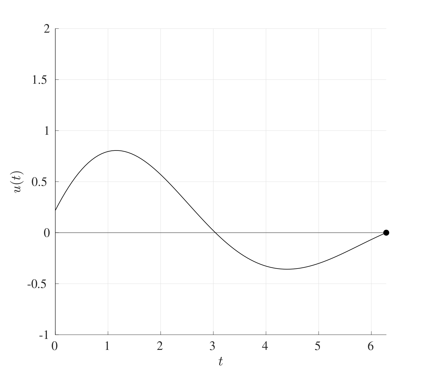 The starting location here happens to be at \(0.2188\) but that is no restricted by the mixed conditions as long as the gradient at the start is \(1\).